Projected Coordinate Systems
So how do we flatten a curved surface? Very carefully.
Hopefully you have all seen or have tried the orange peel demonstration often enough to realize that there is no way to flatten a curved surface without stretching, shearing, and/or tearing it. While we can’t create an undistorted global surface on a flat plane, we do have software that can do complicated math to give us acceptable partial surfaces that strive to preserve specific types of measurements. This math goes on behind the scenes in ArcGIS and is how we convert geographic coordinate systems to projected coordinate systems.
So a map projection is made up of two basic things: a datum that defines how the original curved surface model (spheroid) is pinned to the earth and a mathematical formula that geometrically projects points from that curved surface onto a flat plane.

Projection Specifics
Projections can be visualized as results of a light shining out from the center of a transparent globe, leaving the shadow of the graticule (lines of latitude and longitude) on a flat surface.


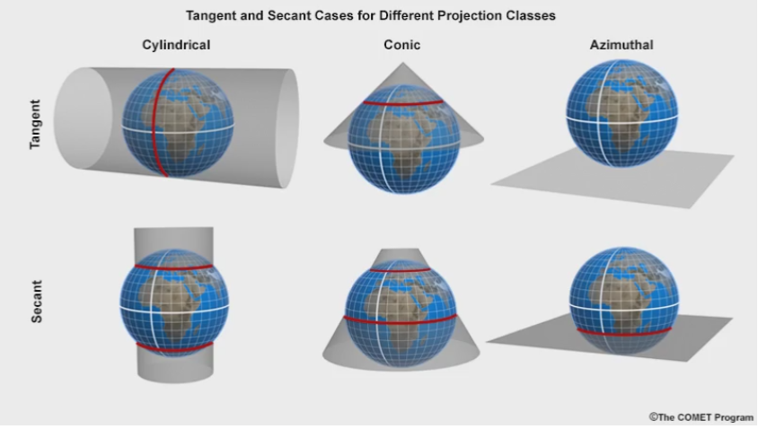
This surface can be a simple plane (an azimuthal projection), a cylinder (cylindrical projection), or a cone (conic projection). Cylindrical projections often depict the whole earth (world maps). Conic projections are appropriate for mapping regions that are wider east west than north south (the continental US versus south America). Azimuthal projections are most often used to depict polar regions.
When flattening a curved surface, the stretching or tearing results in the following typical projection distortions: misrepresentations of area, distance, shape or angle (conformality), or direction. Your job when choosing the appropriate coordinate system for you data and project, is to focus on your area of interest and to choose the math that preserves the metric you are most interested in measuring. For example, if you are measuring migration distances from Alaska to Louisiana, you might choose the North American Equidistant Conic projection.
Projections that preserve area measurements are called “equal area” projections. Equal area projections are useful when mapping relatively small areas (sub-continental). On maps created with equal-area projections each unit of area (m2, acre, km2) at one location covers an equal unit of area at every other location on the map. Preserving area comes at the cost of other metrics we might care about, such as relative scale, angles, direction, or distances.
The least amount of distortion in a projection occurs where the ‘developable surface’ (the cylinder, cone, or plane) touches the globe. In some projections, the projection surface touches in one location, called a Tangent or line of tangency. Projections can also intersect or cut ‘behind’ the globe’s surface creating two locations or lines where the projection surface has no distortion. These lines are called secant lines.

The figure to the right illustrates how compression and extension impact the map as you move away from the secant lines (where the Scale Factor is zero and there is no distortion).
The amount of distortion is accounted for and described in the Projection Parameters as seen below.


The Scale Factor is a measure of the distortion associated with a projected coordinate system. It is the ratio of the measured scale to the true scale at any location on a map. A scale factor of one (SF = 1) means there is no distortion. In the example above, the scale factor of 0.9996 means that there is a compression of the map at the central meridian (the location farthest from the secant lines) of the UTM coordinate system where 100 meters on the earth’s surface will measure 99.96 meters on the map at the central meridian.
To minimize the amount of natural distortion that comes with projecting curved data to a flat surface, we can focus in on a small area of interest. You can imagine that it is impossible to flatten a grapefruit skin without stretching or tearing, but a sugar ant sized piece of paper would sit flat on that grapefruit with no bending tearing or stretching.

The State Plane and UTM projections are regionally limited in extent in order to reduce all distortions as much as possible. This sounds great, but the drawback is that each projection only covers a small areal extent. Calculating between projections is not possible, so for regions of interest that extend beyond a projection’s limit, the distortion will be so great that a different projected coordinate system should be used.

The State Plane Coordinate System is a set of individual projections, each covering a portion of a state. State Pane zones are defined by county boundaries. Each zone is an individual projection; quite a difference in extent compared to the global cylindrical projections!
UTM zones are similar to State Plane zones in that each is an individual projection, small in area, meant to eliminate most distortion. They are equally limited in that we cannot calculate distances or areas between data found in two different UTM coordinate systems. Figure 14 shows one UTM projection, Zone 11. The zone is only 6 degrees wide (the earth is divided into 180 UTM zones), but ArcGIS displays a limited amount of area to the east and west. The distortion gets so unwieldy beyond that point that Arc doesn’t bother displaying it. UTM zones each have a central meridian that acts as it’s east/west origin. It is given the “false easting” value of 500,000 meters instead of 0 to avoid having negative values on the west side of the zone. The Northing origin is the equator. So if you had a UTM coordinate pair of 470,000 meters, 4,610,500 meters could you determine where you were? No. You would know you were 4,610,500 meters north of the equator and 30,000 meters west of a central meridian, but of which zone? It is also important to note, and even a bit confounding, that UTM projections can be applied to any geographic coordinate system. So depending on the datum (in north America alone: NAD 27, NAD 83, WGS 84) this coordinate pair for a specific zone could describe three different locations.
