Random Variables
Pafnuty Chebyshev (1821-1884) coined the term random variable,
defining it as a real variable which can assume different values
with different probabilities
(Spanos, 1999, p. 35). While this was
a simple and intuitive description, it was not rigorous. When Andrei
Kolmogorov (1903-1987) axiomized the study of probability, he prepared
the language and notation necessary to define random variables and
rigorously prove theorems regarding them. We now define a random
variable as a function that assigns the outcome of a random experiment
to a real number.
In the early development of probability theory, only discrete
random variables (although not called random variables at the time)
were considered. Isaac Newton (1643-1727) considered the idea of
equally likely
events defining probability and realized that
this does not necessarily mean that there are a finite number of
cases; there could be infinitely many, including intervals on the
real line. His consideration opened study from discrete to
continuous random variables. Random variables have
distributions which describe the probabilities of their outcomes.
A few common distributions often describe the distributions of
random variables discussed in introductory statistics, including the
binomial, Poisson, geometric, and normal distributions.
Binomial
Blaise Pascal (1623-1662) used binomial coefficients and an
informal use of the binomial distribution to help him solve the
problem of points.
Thus, some historians attribute the development of the binomial
distribution to Pascal. Later, Jacob Bernoulli (1655-1705)
generalized the solution to the problem of points using the
binomial distribution. He named and formalized a description of the
distribution and wrote about it in his Ars Conjectandi (1713).
In addition, he used the binomial distribution to answer other
probability prompts. A key feature of the distribution is a fixed
number of independent Bernoulli trials (trials where the result is a
success or a failure) with the same probability of success. The
term Bernoulli trial
is named for Jacob Bernoulli.
Poisson
The Poisson distribution is named for Siméon-Denis Poisson (1781-1840) who wrote about the distribution in Recherches sur la probabilité des jugements en matière criminelle et en matière civile. The Poisson distribution models the distribution of the number of rare events in a unit of time or space. The context he used was the relationship between the likelihood of convicting a person on trial and the likelihood that they had actually committed the crime. This allowed people to estimate the number of innocent people in jail. Until the time of William Gosset (1876-1937), there had been many attempts to find examples of the Poisson distribution in data, one of which was the number of deaths by horse kicks in the Prussian army. Many attempts were fruitless; however, Gosset found that the number of cells of yeast in each bottle of yeast fluid used by Guinness Brewery to brew beer also followed a Poisson distribution.
Geometric
The geometric distribution is used to describe the number of independent Bernoulli trials up to and including the first success. Little is written about the history of the geometric distribution, possibly because it was developed around the same time as the binomial distribution or because it is a special case of the negative binomial distribution. The negative binomial distribution, which counts the number of trials up to and including the $r$th success, was discussed by Pierre de Fermat (1601-1665) and Blaise Pascal (1623-1662). It was derived and published by Pierre Rémond de Montmort (1678-1719) in 1714. The geometric distribution has many applications, including calculations in the St. Petersburg paradox.
Normal
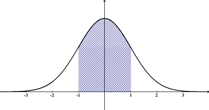
gaussian distribution. Adolphe Quetelet (1796-1874) used the normal distribution to identify fraud in military drafts. Later, Karl Pearson called it the normal curve because he argued it was
normalfor a typical data set to have a normal distribution. Today the term
gaussian distributionis interchangeable with the
normal distribution.